In this project we have worked with the Monte Carlo Localization(MCL) algorithm. The project shows that the MCL is working well in simulation and with some limitations in a physical implementation.
A NXT robot car was build to work in a physical environment. This robot car uses 3 light sensors and 1 compass for the measurements which is essential for the localization. The compass is used to reduce the 3D localization problem(x, y, θ) to a 2D problem (x, y).
We have designed the environment where the car have to locate itself. The environment is a printed gray-scale image, which fits to the properties of the light sensors.
The MCL is implemented in a pc program with a GUI. This program communicate with the NXT through a bluetooth connection. So the car is only used to drive around on the map and measure values.
We have done some successful simulations and test with the implemented system at different states of the development. But we didn't reach all the goals we have hoped and also have some test where the MCL didn't work.
The first experiments was to analyze the sensor accuracy. This gave some of the specifications to the environments we designed and gave a function for each sensors conversions of a gray-level to measure value.
After this we did some experiments with the algorithm in a 1D experiment. The data was analyzed and it was possible to locate the robot car.
Then we moved on to the 2D problem. Where we started out with pure simulation to test the algorithm. Which works as expected, but in the physical test it gave some problems. The problems was coursed by magnetic interference in the lab and the car had difficulties to locate itself.
The problem with the magnetic interference was solved by moving to the location in the lab with the lowest interference.
2 maps was made for the 2D MCL where one of them, a radial gradient was easy to locate on, while the other a more random map was more difficult and in the physical test the last on fail because of ambiguous points.
During the project we worked on a behavior based architecture for the robot car. This should enable the car to stop at the border. But the implementation failed and an simpler implementation.
A goal of the project was to work with the lost/hijacked robot problem, which we never worked with for real. But we tried it with our implementation of MCL, but it never worked.
Another goal was to make the code reusable. This is partly fulfilled, because the project is divided into reusable classes. But the communication between the pc and robot car is build on a very simple protocol, which don't leave many options for extending or changing the functionality of the system.
We are satisfied with the results we have reached in the project even though we have failed to reach all our goals. In the start we was not even sure that MCL would work at all, so we was happy to see how well it actually worked. Another satisfying thing is that we gained some knowhow about a one of the best algorithm for localization, which we can use in our future work.
Anyway it possible to improve the project i several ways. We have made a list explaining some of the possibilities that we would recommend to include in work based on our project.
Friday, January 23, 2009
Wednesday, January 21, 2009
References
[1] Dieter Fox,Wolfram Burgard, Frank Dellaert, Sebastian Thrun; Monte Carlo Localization: Efficient Position Estimation for Mobile Robots.
[2] Frank Dellaert; Dieter Fox; Wolfram Burgard, Sebastian Thrun; Monte Carlo Localization for Mobile Robots.
[3] Maja J. Mataric; Integration of Representation Into Goal-Driven Behavior-Based Robots.
[4] Brian Bagnall; Maximum Lego NXT: Building Robots with Java Brains; Chapter 12.
[5] Dieter Fox; Markov Localization for Mobile Robots in Dynamic Environments (1999)
[6] Jens-Steffen Gutmann; Markov-Kalman Localization for Mobile Robots (2002)
Tuesday, January 20, 2009
Further improvements
Right now the project is at the state "prove of concept". So there is a lot of improvements to the project. We have listed a couple of the important ones.
Autonomic steering, calculation
At this state the robot car can not drive around on it own and find where it's is. It need to be manuel guided around and told when to run the MCL algorithm. The autonomic steering and calculation needs to be implemented, so it's possibly to plant the robot car some random place on the map, and it will go to a certain destination on it's own.
Layer-based car architecture
With a layer-based architecture it would be possible to implement threads with higher priority then the localization thread. Example the thread with highest priority could be "Do not pass the Boarder", so it would overrule the localization thread.
Better/other/more sensors
The sensors used in the project is very dependent the surroundings, as the light, the magnetic interference. They must be recalibrated if the light is changing. Instead of the light sensors there could be used laser sensors. Maybe there should be added some more sensors to get some more measurements to the MCL algorithm.
Cameras could be used and etc. the sensors depends on which environment the robot car has to navigate in.
Without compass
It could be a nice improvement of the algorithm to get rid off the compass. This would transform the MCL2D algorithm to an 3D algorithm. The localization would be rather more difficult and more sensors are needed. If there is a lot of magnetic interference, the compass will completely mess up the measurements. We saw that in the tests.
Adding a better belief function
The actual belief represents just the average of all samples. If the robot is place on a ambiguous map then the average is approximately in the middle of the both clusters. It could be a nice feature to implement a clustering algorithm like k-means to get better beliefs of the real robot position on ambiguous maps.
Comparison to other algorithms
We has only worked with the MCL algorithm, and do not know if it is the best. It would be a good idea to compare the MCL with other algorithms, such as Markov, Kalman and Weiβ algorithm
Monday, January 19, 2009
Test
We had problems to find a place where the compass worked stable. This means there should be a homogeneous and static magnetic field, not necessarily depending on the magnetic field of the earth. The map needs to have the same direction as the compass.
At first the robot is doing a calibration of the compass, then connection to the pc. The map is aligned to compass zero direction. After this phase the robot is placed randomly on the map. This time their are no zero rounds performed to make the algorithm find the robot first and then navigate. The activities are performed both at the same time. As it is shown in the posted video the samples need several rounds of robots driving to build a cluster at the position. There is a second cluster with is close to the one at the real position. After some more steps the cluster surrounds the real robot position.
The MCL2D algorithm worked well in an interactive environment and was able to localize the robot after some rounds.
The results in the second map are not as good as the one in the other. In the experiments did on the second map were always more then one cluster, the robot was lost in a few tests. Sometimes it worked well. It is to say that the second map has to much ambiguities to localize proper. We tried to spread some samples (about 5-20%) in the map to find the robot again when it was lost while the localization process. After this change the algorithm didn't work well anymore. So the change was skipped.
Saturday, January 17, 2009
Programming the robot car
The robot car have only a few functions, which is:
- Communicate with the PC through bluetooth.
- Drive as ordered from the PC.
- Measure the light levels with the 3 light sensors.
- Measure the direction with the compass.
- Stop at the border.
Behavior-based implementation
All the function except the stop at the border is a sequence of things which have to be executed in the right order. But the stop at the border have to run parallel with this sequence because it have to stop the car if it reaches the border.
For this reason it will be appropriate to use behavior-based architecture with a thread for the sequence and one for the stop at the border.
Before the threads are started there will be calibration of the compass and connection to the PC.
The sequence have to receive orders from the pc, complete the order(turn and drive), measure the light levels at the destination and send these values back together with the compass value.
The stop at border have to stop the car if it detect the black color i the direction it is driving. This have to change the order so the car won't drive any further when it returns to the sequence thread.
The implementation was based on Maja J. Mataric's article [3] and the work we made in lab lesson 10. Because the car have different functions this time we rewrote the car class and the behavior class. The new car class was based on the CompassPilot class, which had the functions we needed to navigate on the map.
Based on this we implemented the two threads and started them in a main program. But when we executed the program we got an exception. After some work to avoid the exception we decided to give up the behavior-base architecture.
One thread implementation with stop at the border
The failure of the behavior-base implementation lead to a simpler implementation with only one thread which structure was build on the structure of the sequence thread mentioned above.
In addition the immediateReturn opportunity of the rotateTo og travel functions, and while the car was traveling we made the program execute a while loop were it was looking for the black color, and stop the car if the color was detected.
This program was executeable and we made some tests with it. In these tests the car didn't always stop rotating or driving forward. By removing the immediateReturn option the car was driving more stable, even though we had some trouble with the magnetic field was changing very quickly on the map at some positions in the lab(more about that in the description of the tests).
Removing the immediateReturn also removed the possibility to detect the black border.
One thread implementation without stop at the border
The code for the robot car have yet another time been simplified with the removal of the detection of the border. But now we have a working robot car with exception of the boarder detection. The consequence of this is that we can't drive blind around on the map, but have to look at the cars position on the map before we gives a order to make sure the car isn't driving out of the map.
The previous implementations had a calculation of a direction according to a local north which was initialize in the beginning. But this was removed because it might be the source to some errors we experienced. The removal of this made the code even more simple, but as consequence the map have to be adjusted to the real north according to the compass.
The implementation of the robot car included 3 classes listed and linked to here:
- MCLcar.java
- carBT.java
- myOrders.java
MCLcar.java is preforming initialization and the sequence described above.
carBT.java is the functions that makes the bluetooth connection possible.
myOrders.java is use to pass the orders received form the pc through bluetooth to the MCLcar.java.
pc program
GUI

The GUI gives a overview of the samples (green dots), and the average of the samples is showed with a red circle, on the map. This data (green dots and red circle) is updated each time the robot car moves, and they are showed in the top console. Where to the robot car should move is done manuel by sending the distance and angel to turn. The map loaded/showed by the GUI is also the one used in the MCL algorithm.
MCL2D algorithm implementation
The implementation of the MCL2D algorithm is object orientated. The basis for the algorithm is
the sample class with consist of the position p = (x,y,t) and the importance i.
Furthermore there is the implementation of the MCL algorithm which is the class called MCL.
There are several constructors with are able to set the important variables:
samplescount = number of samples used in one round.
xrange and yrange = maximal range of the physical map with respect to the maps direction.
nx and ny = pixelwise resolution of the map representation.
In the beginning the function "initialise" makes it possible to set the samples randomly and
equally distributed on the map which is represented as a picture.
The function "setAllTheta" makes it possible to set all the angles of the samples with respect to
the direction to the same values.
The belief is represented by the function "expectedPosition" with calculates the average of the
samples, it could be a good idea to use other (clustering-) methods to calculated the belief.
The most important function is the "update" function which updated the samples and the belief.
The function gets the offset of the robot as well as the actual sensor readings and the uncertainty.
Implemented classes
- window.java (main)
- myMeasurements.java
- MyCanvas.java
- bluetooth.java
- MCL.java
- MyImage.java
- Position.java
- Sample.java
Bluetooth
The bluetooth connection between robot and pc is based on an exchange of needed data for the localisation. The car- as well as the pc side gives a tuple of integers back.
The cars side: (dx, dy, theta, s1, s2, s3)
dx and dy are the driven offsets of the car, the change of the cars position since the last data exchange. theta means the absolute orientation of the car with respect to the map. s1, s2, s3 are the sensor readings which are necessary for the localisation.
The pc side: (dtheata, drive)
The pc side gives a turn and a certain distance to drive to the robot.
Every communication phase between robot and pc takes exactly eight steps. Six steps for the car and two steps for the pc. Just integers are sent, to make it as easy as possible.
Our experiments with the bluetooth showed that this way of exchanging data is very stable. The connection didn't break down after 10 minutes of exchanging data between robot and pc.
This shows that the implemented bluetooth class is satisfied for the tasks.
Wednesday, January 14, 2009
Simulating in a physical world
The two different maps used in the simulation for the MCL2D algorithm are also used in the simulation in a physical world. The maps were printed in the size 841 mm x 594 mm on a plotter.
The algorithm is calibrated on the used gray scales. The robot is placed on the map with a relative direction of zero degrees and on several, different positions. In these first experiments the robot is not interacting with the world. The world is also static. To follow the test we put a picture of the physical world and the map representation with samples together. As it is obviously, by knowing about the relative direction, the first map is still unique, the second is not.
The first map:
The algorithm is performing an amount of rounds before it is obviously that the samples will build a cluster at a certain position on the map. After all the tests there was always a cluster at the right position which wins after several steps.
The test show that the MCL2D algorithm works quiet accurate in the physical environment. Most of the approximations don't have an strong effect on the error.

In this experiment the robot car is set in the right lower corner. The MCL2D algorithm developed to cluster of samples. The cluster at the right position is growing while the other one is shrinking. After a certain amount of steps the algorithm was able to localise the robots position.

In this experiment the robot car is set in the right upper corner. The MCL2D algorithm developed to cluster of samples at the two upper corner of the map. The cluster at the right position is growing while the other one is shrinking. After a certain amount of steps the algorithm was able to localise the robots position.

In this experiment the robot car is set in the left upper corner. In this case the MCL2D algorithm doesn't developed different clusters of samples. The cluster at the right position is growing quickly. After a certain amount of steps the algorithm was able to localise the robots position.
The uniqueness of the map helps the algorithm to find the right point without following a trajectory.
The second map:
The ambiguity of the second map is obviously a problem for the algorithm. To solve this problem the robot has to change its position at one point in the experiment. After all it's possible to say that the MCL2D algorithm works well on the second map. There was always a cluster at the right position with a strong probability and a lot of samples. Most of the chosen position where localised in the experiments

In this experiment the robot car is set in the right upper corner. The MCL2D algorithm developed two clusters of samples at different positions with approximately the same expected sensor readings. The cluster at the right position is growing while the other one is shrinking, but it took a lot of steps in comparison to the first map. After a certain amount of steps the algorithm was able to localise the robots position.

In this experiment the robot car is set in the left lower corner. The MCL2D algorithm developed two clusters of samples at different positions with approximately the same expected sensor readings. The clusters have a big concurrency so no one of them is able to get all the samples.
It's necessary to drive a trajectory with the robot to get more information about the actual position and to localise the robot.
A trajectory is needed to solve the ambiguity of the map.
Tuesday, January 13, 2009
Simulation and drawing
Simulated experiments with MCL2D
The combination of the graphical user interface and the MCL2D class is established. The following experiments show how the MCL2D algorithm works on different kind of maps. The first map is in respect that we know about the relative angle to the map, unique. The second one has several ambiguous points as it's possible to see in the images. The red blob is a representative for the expected position of the actual MCL-state (the average of all sample positions), the green circles are the samples at their certain position and the blue blob is the position of the robot, which we type into the simulation. The robot never moves in the simulation.
The sensor inputs is simulated by using the function which estimate the meassured value from a position. This is the same function which is used to estimate the measurements of the samples. Because the same function is used it's possible to have exact matches.
We expect that the samples will go to the blue blob, because they want to reduce the error of the comparison with the real- and the expected sensor readings. Because of the uniqueness in the first map there should be one cluster of samples around the simulated position. The second map could show several clusters.
This experiment shows that the MCL-algorithm seems to work accurately. The samples clumb after several steps at the simulated position. The endpoint will not be smaller because of the uncertainty in the algorithm

This experiment has ambiguous points. These points give the same sensor readings. After some steps the samples clumb at four different positions with a higher probability and more samples at the simulated position. After several steps the samples build a cluster at the simulated position.

After some simulation experiments it's possible to say that the algorithm works accurately. None of the test runs with image one didn't find the simulated position. The test runs with map two showed that the samples always clumb after several steps at one of the possible positions.
This gives the conclusion: It should be possible to follow a robot correctly on these maps with a very high probability. It should be possible to use the algorithm in an physical world.
Monday, January 12, 2009
Probabilistic Localization
Navigation
Navigation is the process of keeping the position or the trajectory to a goal in mind (this means in the memory of the robot or a computer). There are to main ideas: localization (Pos.) + path planning and direct computing of the course to the goal.
For these things there are to things necessary: A model of the world (map) and the sensor readings. There are two types of maps: topological and geometrical. We will deal with a geometrical (an image). There are a lot of arguments for probabilistic localization:
probabilistic formulation of the localization problem:

a.) continuous, single hypothesis (e.g.Kalman)
b.) continuous, multiple hypothesis (e.g. Kalman)
c.) discrete, multiple hypothesis, geometrical map (e.g. Markov, Monte Carlo)
d.) continuous, multiple hypothesis, topological map (e.g. Kalman)
Monte-Carlo-Localization (MCL)
Ordinary localization methods like the Markov-Localization need many resources to compute the approximation of the localization belief.
Because of the discretization of the map there is no limit of making the result more precise. For this reason we need a method with a finite number of belief representations. This beliefs are called samples in the following parts of the description.
These points are characteristic for the used Monte-Carlo-Localization:
The Samples
A Sample consist of an expected position (x,y,θ) as well as an importance factor.
The Algorithm
initial belief: set of k samples with equally distributed importance factors 1/k.
known: in the pure setting just the sensor readings. Here with the relative orientation to the map
goal: compute a peak at the real robot position.
Actualization of the belief:
1. choose randomly a sample out of the set of samples with respect to the importance factor.
-> position L(T-1)
2. pick out the next position with the robots action-model P(L(T) | A(T-1), L(T-1) ).
-> position L(T)
3. give the sample a new unnormalised importance P(S(T) | L(T)) by the sensor-model an put it in the new samples set.
4. repeat step 1.-3. k times and normalize the importance of the new samples set.
Closer look at the steps
1. choose randomly a sample out of the set of samples with respect to the importance factor.
-> position L(T-1)
Roulette wheel selection (the higher the importance of a certain sample the bigger the area on the wheel). A point on the wheel is randomly chosen. The higher the importance the higher the probability to be chosen. It is shown in the figure:

2. pick out the next position with the robots action-model (which transforms the tacho counters into an position offset) P(L(T) | A(T-1), L(T-1) ). The tacho counters at time T are represented by A(T).
-> position L(T)
Choose the following position which is produced by the error function of the action-model. The new position of the car is changed with respect to the tacho counters and the action-model. The following position is set with a uncertainty. Shown in the figure:
 3. give the sample a new unnormalized importance P(S(T) | L(T)) by the sensor-model and put it in the new samples set.
Sensor readings: expected Sensor reading contra real sensor readings, the higher the different the lower the probability of the belief. Hopefully the samples clump at he right position.
A = (100.0-|realsensorA - expectedsensorA|)^10
B = (100.0-|realsensorB - expectedsensorB|)^10
C = (100.0-|realsensorC - expectedsensorC|)^10
newimportance = (A+B+C)^10
The figure shows a robot with laser sensors with a belief distribution. The more accurate the sensors are the better ans more precise the belief is (laser are more accurate the sonar sensors).
 Pros and cons
+ very efficient with about 100 samples
+ robust even with less good maps
+ any-time: more resources = more samples
- high concentration of the samples, problems with a kidnapped robot
Navigation is the process of keeping the position or the trajectory to a goal in mind (this means in the memory of the robot or a computer). There are to main ideas: localization (Pos.) + path planning and direct computing of the course to the goal.
For these things there are to things necessary: A model of the world (map) and the sensor readings. There are two types of maps: topological and geometrical. We will deal with a geometrical (an image). There are a lot of arguments for probabilistic localization:
Random noises on sensor readings, the physics of a robot are never certain.
There is a belief of the real position (different representations), actualization of the belief with the robot physics and the sensor readings.

a.) continuous, single hypothesis (e.g.Kalman)
b.) continuous, multiple hypothesis (e.g. Kalman)
c.) discrete, multiple hypothesis, geometrical map (e.g. Markov, Monte Carlo)
d.) continuous, multiple hypothesis, topological map (e.g. Kalman)
Monte-Carlo-Localization (MCL)
Ordinary localization methods like the Markov-Localization need many resources to compute the approximation of the localization belief.
Because of the discretization of the map there is no limit of making the result more precise. For this reason we need a method with a finite number of belief representations. This beliefs are called samples in the following parts of the description.
These points are characteristic for the used Monte-Carlo-Localization:
Random based, finite number of samples, importance factor to change the probability distribution.
A Sample consist of an expected position (x,y,θ) as well as an importance factor.
The Algorithm
initial belief: set of k samples with equally distributed importance factors 1/k.
known: in the pure setting just the sensor readings. Here with the relative orientation to the map
goal: compute a peak at the real robot position.
Actualization of the belief:
1. choose randomly a sample out of the set of samples with respect to the importance factor.
-> position L(T-1)
2. pick out the next position with the robots action-model P(L(T) | A(T-1), L(T-1) ).
-> position L(T)
3. give the sample a new unnormalised importance P(S(T) | L(T)) by the sensor-model an put it in the new samples set.
4. repeat step 1.-3. k times and normalize the importance of the new samples set.
Closer look at the steps
1. choose randomly a sample out of the set of samples with respect to the importance factor.
-> position L(T-1)
Roulette wheel selection (the higher the importance of a certain sample the bigger the area on the wheel). A point on the wheel is randomly chosen. The higher the importance the higher the probability to be chosen. It is shown in the figure:

2. pick out the next position with the robots action-model (which transforms the tacho counters into an position offset) P(L(T) | A(T-1), L(T-1) ). The tacho counters at time T are represented by A(T).
-> position L(T)
Choose the following position which is produced by the error function of the action-model. The new position of the car is changed with respect to the tacho counters and the action-model. The following position is set with a uncertainty. Shown in the figure:
 3. give the sample a new unnormalized importance P(S(T) | L(T)) by the sensor-model and put it in the new samples set.
Sensor readings: expected Sensor reading contra real sensor readings, the higher the different the lower the probability of the belief. Hopefully the samples clump at he right position.
A = (100.0-|realsensorA - expectedsensorA|)^10
B = (100.0-|realsensorB - expectedsensorB|)^10
C = (100.0-|realsensorC - expectedsensorC|)^10
newimportance = (A+B+C)^10
The figure shows a robot with laser sensors with a belief distribution. The more accurate the sensors are the better ans more precise the belief is (laser are more accurate the sonar sensors).
 Pros and cons
+ very efficient with about 100 samples
+ robust even with less good maps
+ any-time: more resources = more samples
- high concentration of the samples, problems with a kidnapped robot
Thursday, December 18, 2008
Environment design (2D maps)
The primary consideration of this part is to make a map which can be represented digital with a high accuracy.
We was thinking about taking a picture of the world where the car is driving, and use it as this representation. But we quickly concluded that the picture had to be taken in a very precise angle. So we decided to draw our own maps on a pc, thus the digital representation is made and we have to print it out.
The car have to drive around on the map, so the map have to be larger than a A4. An A1 paper will give some space to drive on and still it is possible to make the map on a plotter. A A1 paper have the dimensions (landscape) 841 times 594.
Properties of the maps
The light sensors only measure the level of reflected light and no colors, thus the map is only read as gray values so the easiest way to make it is with gray values.
In the previous test we saw that the sensors had problems to distinguish the high gray values. So we will only use the following colors on the maps we make:
# - color level
0 - 0 (border)
1 - 20
2 - 40
3 - 60
4 - 80
5 - 100
6 - 120
7 - 140
8 - 160
9 - 180
10 - 200
11 - 220
The robot must know where the border of the map is, so the map have to have a unique gray-level at this border. Thus the black color(0) is only used for the border. The black color is used because it is easy to distinguish it from the other colors.
The border is made 3 cm wide so we are sure that the robot will detect it.
The sensors can't detect high details, so we will only use 1 dot per mm in the maps. Thus the images must have a resolution of 841 x 594 pixels.
This leads to two maps which will be used in the following work. These are named map 2 and map 3 and are described more in the following sections. Map 1 was a discarded because we thought it would not work.
Map 2
Map 2 is mad by drawing a lot of rectangles with the gray levels listed above. The rectangles are of random size and place random. But the map is made by a human, so it will never be total random. The map is made of rectangles with a width of at least some pixels, because the sensors can't detect high details.
In the end the black border was add so it's possible to make the car stay on the map.
 This map can have ambiguous points, which is point where the MCL won't be able to distinguish. So this map might be difficult to get the MCL to work on. But when the car is moving it should be possible to distinguish the points because there is no repeated sequence.
Map 3
Map 3 is made with a radial gradient with center in the middle of the map and a black border outside.
In this map each position is unique(when the compass gives the angle), which makes it a easy map to make the MCL work on. An even bigger advantage of the map is that the local maximum of probabilaty is the global maximum, so the longer the robot car are from a point the lower importans it will get.
 Map 3 is not very realistic map but it's a good map to start on, because of it's properties.
Friday, December 12, 2008
1D Monte-Carlo Localization
With a function to convert from color values to light sensor values in place, and code for a 1D Monte-Carlo localization(MCL) we were ready to test the converting function and the 1D-MCL.
This test was also used to decide if the converting function found in the Light Sensor Test section was accurate enough. So there have been switch back and forth between these tests.
Method
We have printed a ramp(shown below) with a length of 25 cm on an A4 paper.

The MCL algorithm is running on the pc, while exchanging data with the car via bluetooth. But the software to send commands to the car and receive data from the car is not developed yet, thus we moved the car around by hand, and then manually wrote the measured values into the program.
In this test we only use one sensor.
The code is devided into 3 classes which is written below here. The Sample class is used to make samples with a x position and an importance. The MCL class have all the functionality of the MCL and the MCLMain is used to write input and get ouput back from the MCL.
We were runing a serie of experiments, and the code linked to here is the last one we ran.
MCLMain.java
MCL.java
Sample.java
Experiments
Experiment 1
At this expriment we moved the car arround with the diffrent convertionfunctions found in the Light Sensor Test section. But the MCL localized the robot a up to a few cm wrong(with the piecewise linear function). So we looked into the MCL to find out why i was so.
Experiment 2
When we looked at the importance of the samples they were almost the same size, so we decide to ad a power-function to calculation of the importance. In this experiment we used a power of 10.
Because we wanted to make sure that the MCL were working we let all the measurements be the same - like the car was at one x-position(15) and measured the same each time(48).
We used 100 samples and ran 11 cycles trough the MCL.
At the end the end we printed the positions and importance of the samples and analyzed them i a matlab program(linked to below).
measurementAnalyzing.m
After the 11 cycles of the MCL the histogram of the sample position is shown below here. You can see that the most samples is located a little below 16. Which shows that the samples is moving toward the actual position(15).
 The figure below shows the importance of the samples as function of their position. It's easy to see that the samples around 15 have the highest importance. Which made us conclude that a few more cycles would make the points move even more toward the actual position.

Experiment 3
Now we have a working MCL, but we were a little concerned about the power of 10. A downside of it could be that the MCL could move toward a wrong position and then not be able to correct it.
So we turned the power down to 2 and added more samples so we now were using 1000 samples. Everything else was as Experiment 2. And the output was analyzed in the matlab program.
The histogram of the x-positions below shows that the samples is much more widely placed on the map. But even though there is the highest amount of samples at 15, so it is working.

The importance as function of the position is much more flat than before and there is some bumps in the curve. But the highest importance is at 15 as expected.

Experiment 4
To see if the results of Experiment 3 was improving if the MCL was running more cycles we made it run for 111 cycles.
This results in that all the samples have their x-position inside 15 +/- 2,5. So the samples is moved much closer to the actual position. (the reason that the bars are not higher is that the samples still are separated into 50 bars, but the bars is only covering 5 cm were they before were covering 25 cm).
 The importance as function of the position(shown below) ave become much more sharp and there is no bumps on the curve. So it is possible to achieve about the same precision with power 2 as 10, but it requires more samples and more cycles.

Conclusion
The 1D MCL is working and the sensors seems to be accurate enough to make it posible to find the posistion in the 1D-map. More experiments must be made on more advanced maps to determind the best parameters for the MCL. Is it high power and fast tracking or is it a low power and slow tracking.
This test was also used to decide if the converting function found in the Light Sensor Test section was accurate enough. So there have been switch back and forth between these tests.
Method
We have printed a ramp(shown below) with a length of 25 cm on an A4 paper.

The MCL algorithm is running on the pc, while exchanging data with the car via bluetooth. But the software to send commands to the car and receive data from the car is not developed yet, thus we moved the car around by hand, and then manually wrote the measured values into the program.
In this test we only use one sensor.
The code is devided into 3 classes which is written below here. The Sample class is used to make samples with a x position and an importance. The MCL class have all the functionality of the MCL and the MCLMain is used to write input and get ouput back from the MCL.
We were runing a serie of experiments, and the code linked to here is the last one we ran.
MCLMain.java
MCL.java
Sample.java
Experiments
Experiment 1
At this expriment we moved the car arround with the diffrent convertionfunctions found in the Light Sensor Test section. But the MCL localized the robot a up to a few cm wrong(with the piecewise linear function). So we looked into the MCL to find out why i was so.
Experiment 2
When we looked at the importance of the samples they were almost the same size, so we decide to ad a power-function to calculation of the importance. In this experiment we used a power of 10.
Because we wanted to make sure that the MCL were working we let all the measurements be the same - like the car was at one x-position(15) and measured the same each time(48).
We used 100 samples and ran 11 cycles trough the MCL.
At the end the end we printed the positions and importance of the samples and analyzed them i a matlab program(linked to below).
measurementAnalyzing.m
After the 11 cycles of the MCL the histogram of the sample position is shown below here. You can see that the most samples is located a little below 16. Which shows that the samples is moving toward the actual position(15).
 The figure below shows the importance of the samples as function of their position. It's easy to see that the samples around 15 have the highest importance. Which made us conclude that a few more cycles would make the points move even more toward the actual position.
Experiment 3
Now we have a working MCL, but we were a little concerned about the power of 10. A downside of it could be that the MCL could move toward a wrong position and then not be able to correct it.
So we turned the power down to 2 and added more samples so we now were using 1000 samples. Everything else was as Experiment 2. And the output was analyzed in the matlab program.
The histogram of the x-positions below shows that the samples is much more widely placed on the map. But even though there is the highest amount of samples at 15, so it is working.

The importance as function of the position is much more flat than before and there is some bumps in the curve. But the highest importance is at 15 as expected.

Experiment 4
To see if the results of Experiment 3 was improving if the MCL was running more cycles we made it run for 111 cycles.
This results in that all the samples have their x-position inside 15 +/- 2,5. So the samples is moved much closer to the actual position. (the reason that the bars are not higher is that the samples still are separated into 50 bars, but the bars is only covering 5 cm were they before were covering 25 cm).
 The importance as function of the position(shown below) ave become much more sharp and there is no bumps on the curve. So it is possible to achieve about the same precision with power 2 as 10, but it requires more samples and more cycles.
Conclusion
The 1D MCL is working and the sensors seems to be accurate enough to make it posible to find the posistion in the 1D-map. More experiments must be made on more advanced maps to determind the best parameters for the MCL. Is it high power and fast tracking or is it a low power and slow tracking.
Thursday, December 11, 2008
Light Sensor Test
The goal of this part is to estimate the accuracy of the light sensors and the difference between them. I addition we want to end up with a function, which converts a color value to an light sensor value.
Preparation
To test the the light sensors we used 2 gray bar images(shown below, they will be referred to as respectively step8 and step15).

 The color of each color bar is shown in the spreadsheet below(the id refers to the number printed on each bar in the images and the color value of each bar is rounded ):
 The images were printed on a A4 paper with a standard laser printer, which made the quality of the print a bit noisy. The images were stretched to fill out almost the hole paper, so the bars were as big as possible.
Measuring the sensors
Method
The sensors were placed on the car at their final positions, so there is no error in the angle or distance to the surface below the sensor.
Both tests where made by moving the car around, so one sensor at a time where measured at each bar in the images. Below is a image of the car measuring one of the sensor values on one of the color bars.

To run the test the following code were implemented in the NXT. It use the 3 color sensors and write their values to the LCD.
----------------------------------------------------------------------------------------------------------------------------
import lejos.nxt.*;
public class SensorTest{
public static void main(String [] args) {
LightSensor light1 = new LightSensor(SensorPort.S1);
LightSensor light2 = new LightSensor(SensorPort.S2);
LightSensor light3 = new LightSensor(SensorPort.S3);
while (! Button.ESCAPE.isPressed())
{
LCD.clear();
LCD.drawString("S1: ",0,0);
LCD.drawInt(light1.readValue(), 3, 4, 0);
LCD.drawString("S2: ",0,1);
LCD.drawInt(light2.readValue(), 3, 4, 1);
LCD.drawString("S3: ",0,2);
LCD.drawInt(light3.readValue(), 3, 4, 2);
LCD.refresh();
try { Thread.sleep(100); } catch (Exception e) {}
}
LCD.clear();
LCD.drawString("Program stopped",0,0);
LCD.refresh();
} }
----------------------------------------------------------------------------------------------------------------------------
Expectations
We hope there is a linear function between the color value printed on the paper and the value we measure, because it will make the conversion easy. If not we may see if the error is small enough to be neglected.
Results
The measurements gave the following result:
 The results of the measurement on the step15 image are plotted on the following figure.
 By looking at the measured values it was obviously that the sensor could not distinguish the difference between the light gray colors - There is almost no difference between the last 3 values of each sensor. In the other end the black have a large jump to the next color bar compared to the other steps.
It's clear that light sensors gets different measurements for the same color. Which means that we have to implement a function for each light sensor.
On this background we had to estimate a function to convert a color to a sensor value. To do this we omitted the first value and the 2 last color bars and then made Microsoft Excel try to give us different functions as seen below.
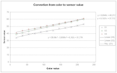
We tried to make a linear function for the conversion, but it was not accurate enough.
So we tried with a polynomial estimation, but still it failed to be accurate enough. So we ended up with the conclusion that we have to use a piecewise linear function, with one piece between every measurement.
Another thing about these results is that 15 levels may have too little difference to be distinguished. So a little less may be prefferred.
Conclusion
It was not possible to make a linear function to convert a color value to a sensor value, so we ended up using a piecewise linear function.
The sensor can not distinguish the light colors from each other. So these cannot be included in the color range used in a map.
Thursday, December 4, 2008
Pretest Bluetooth
For testing the bluetooth communication, the included samples from LeJOS was used (BTSend.java and BTReceive.java). The test was successfully there was made a connection between the PC and the NXT, and data was exchanged.
But there was a little problem, if the NXT is waiting to long for establish a communication, it will make a exception. We can't find the reason why. But its solved by connecting before the time out.
The bluetooth communication is working, and its should not be that big a problem to work with these class', and make them fit our project.
Building the robot
The robot needs three light sensors and one compass, as it is now. It has to be stable. The main idea for the robot are from the manual LEGO Mindstorm Education Base set 9797. As you can see at the pictures below, the lower structure of the robot car is similar to 9797.

Picture of the robot

Drawing of the sensor placement, sensor 1-3 is light sensor. Seen from the top
The light sensors is stabilized so the the vibration of them is minimize and the measurement is more stable. The positions of the light sensors should be as far as possible (without making the construction unstable and to big for the map) from the robot center. This is to make the sensors change more while turning the robot. Otherwise the shouldn't be to far from the robots center because we would easily touch the border of the environment, which is not anymore represented in the map.
The NXT only has 4 sensor ports, one of those has to be used for the compass, which leads to three ports for the light sensors. These are placed in the corners of the robot car and as vertical as possible. Below is a drawing of placement. The center of the car is between the front wheels. If there were more sensorports we would use them, because the algorithm gets more precise the more sensors it has.

Drawing of the sensor placement, sensor 1-3 is light sensor. Seen from the top
Plan - steps to go through
- Analyzing light sensors: printing a gradient-map and a step-map. And see how the sensors react and get an idea of the uncertainty in the light sensors by using more than one sensor.
- Read papers about MCL.
- Write detailed description of the algorithm.
- Write detailed description of the problem.
- Map representation in java
- How to use the compass.
- How to use the navigation class.
- Learn to use the Bluetooth.
- Specify the API’s in the system. Take into account that the system or parts of it should be able to be use in a later project.
- Program the algorithm, Bluetooth communication, car sensoring, PC GUI.
- Specify 1- dimensional experiments.
- Make a 1-dimensional experiment.
- Specify full-scale experiments.
- Design a map or more maps
- Make full-scale experiments.
- Build the robot
Future work:
- When the robot have found it’s position it drives to a specified position.
Problems:
- Bluetooth connection
- GUI
- Map-representation.
- Sample position update.
- Importance update.
Thursday, November 27, 2008
End course project - Finding project
End course project - Finding project
Brainstorm
1) Monte Carlo Localization
The robot is supposed to localize itself in a known world, by having an internal geometrical representation of the surrounding.
2) Balancing robot
Deal with the problem of a two wheeled balancing robot. Extend the idea of using a PID controller to full state control. And apply a remote control for tilting the robot so its driving forward or backwards.
3) Evolution
Exchange genes for solve a task better.
4) Navigation
Make four robots work together to move from a specified position to a specified target.
Three projects in detail
We have excluded no. 3, because we didn't have a good idea for a project including the evolution theory.
1) Monte Carlo Localization
How should a map look like for easy localization?
Detailed measurement of the light sensors.
How to design a robots which is able to apply accurate light sensor measurements.
Finding out, how the communication between PC and NXT works.
PC program with visual interface showing the possible position of the NXT. At the same time the PC is doing the heavy calculation.
NXT and PC algorithm programming.
Goal-experiments:
- Ordinary localization: from random samples to the robot position.
- Lost/hijacked robot problem: robot was found and set to another position. Will the samples find the new position?
- Tracking: samples already know the robots position and try to follow the robot.
needed parts:
- 1 ordinary NXT package
- 3 Light Sensors
- 1 Compass
- Landscapes
2) Balancing robot
Detailed mathematical analysing of the robot physics for the fullstate feedback control description.
Building the robot, maybe different configurations.
Try to apply the bluetooth communication between PC and NXT for the remote control.
Goal-experiments:
- Balancing time of the robot while starting in an vertical position.
- Testing the remote control.
needed parts:
- 1 ordinary NXT package.
4) Navigation
Find an appropriate path model.
Determine the distances between the robots while using local sensors.
Dealing with the communication between the robots.
Try using a Kalman filter.
Goal-experiments:
- The point to point navigation (while obstacle avoiding).
- with and without Kalman.
needed parts:
- 4 ordinary NXT packages.
Choosing Project:
We have chosen the project no. 1 (Monte Carlo Localization). Because the project includes many of those subjects we have been through in the course. Example navigation, behavior layers and more may come. Project 4 was excluded because we couldn't see how to measure the distance between the robots.
Schedule for next time:
- How to make a map, using plotter etc.
- Build robot.
- Color test for light sensor
- Overall schedule for project.
Subscribe to:
Posts (Atom)